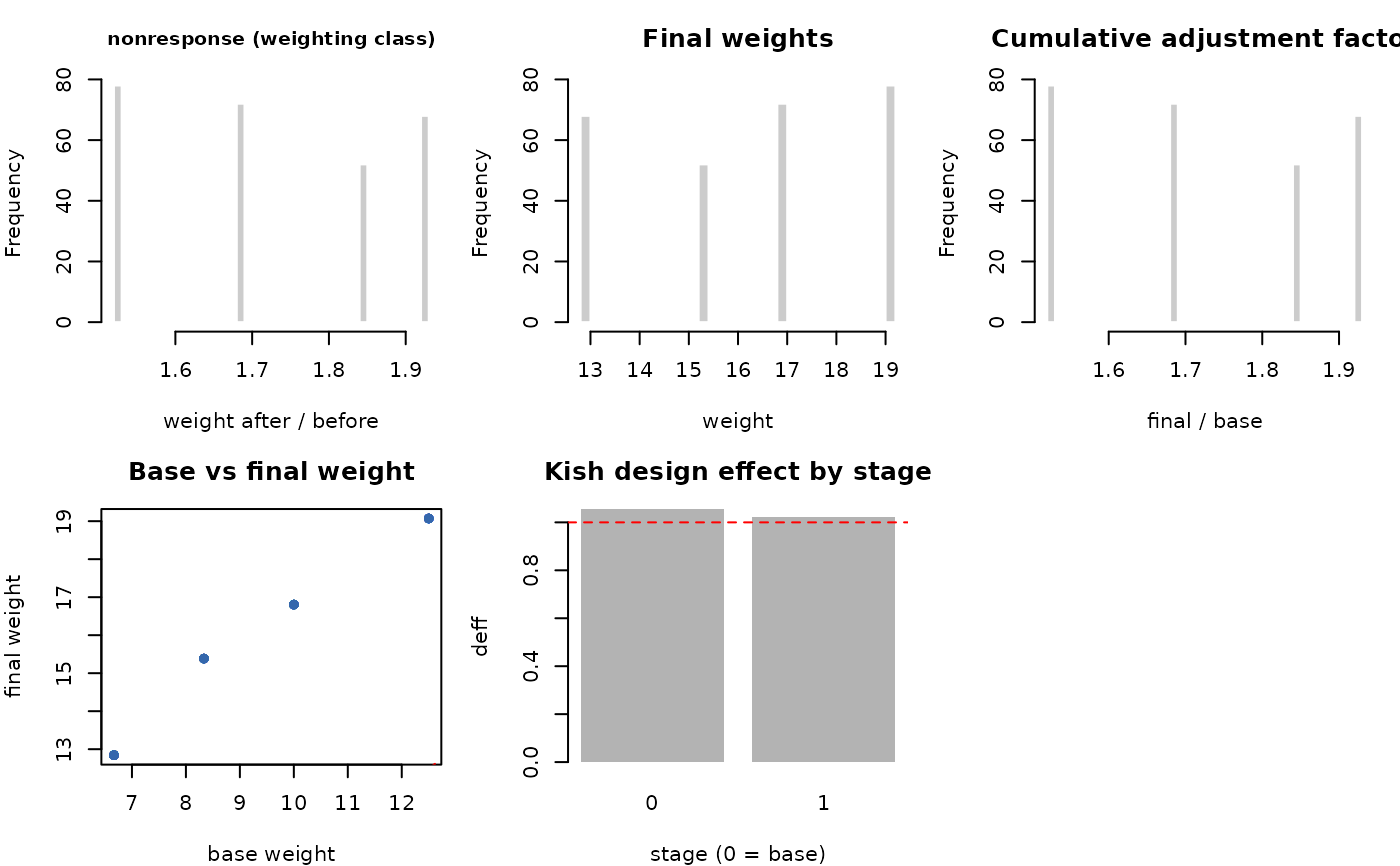
Diagnostic plots for the weights — plot.prepped_weighting

Draws the weighting cascade: one histogram of the adjustment factor per step, plus a four-panel summary of the final weights, the cumulative factor, base against final weight, and the design effect by stage. Base graphics only, no dependencies. Use it after prep() to see how the weights moved, where summary() tells you by how much.

Usage

# S3 method for class 'prepped_weighting_spec'
plot(x, type = c("all", "factors", "summary"), ...)

Arguments

x: a prepped object (output of prep()).
type: "all" (default): per-step adjustment-factor histograms PLUS the summary panel (final weights, cumulative factor, base vs final, deff by stage), all in one grid. "factors": only the per-step factor histograms. "summary": only the summary panel.
...: ignored.

Value

Invisibly, the prepped object x. Called for its side effect of drawing the diagnostic plots described above.

Examples

fitted <- weighting_spec(sample_survey, base_weights = pw) |>
  step_nonresponse(respondent = responded, method = "weighting_class", by = "region") |>
  prep()
plot(fitted)